
Solid quantitative reasoning skills (logic, mathematics, and statistics) are at the core of understanding and interpreting many sustainability concepts and are required for making sustainability-related decisions. The USE Math project develops and disseminates classroom-ready activities that engage students in authentic experiences within the context of sustainability.
 A paper written by Bob Day and me about our Carbon Game will appear in an upcoming issue of INFORMS Transactions on Education. An advance version is available from the journal’s website at http://pubsonline.informs.org/doi/abs/10.1287/ited.2017.0171 .
This is a classroom game aimed at teaching students about some of the basics of energy markets, the use of regulation to induce environmental benefit, and development of mathematical strategies including connections to mathematical/O.R. concepts such as game theory and the news-vendor problem. While the game is fairly simple to set up and play, the results can be somewhat complex. In the paper, we define quantitative metrics for evaluating the quality of student player performance on ranges of rational/irrational and selfish/cooperative.
The quantitative background assumed of student players is minimal. A simple (non-calculus) mathematical modeling course would suffice and most of the benefits the game provides will accrue to such students. Students with a stronger O.R. background will be able to capitalize on that to develop more sophisticated mathematical strategies. This will provide even richer post-game discussion and analysis opportunities for students and instructors.
The article contains supplemental materials to guide the instructor in facilitating the game. It is our hope that others will find our game useful as an active learning experience for their students, and that some may take the game and its analysis in new and exciting directions. Enjoy!
(Here are a couple of old posts I wrote about the game: 1) a talk I gave 2) a poster about it .)
Bicycle sharing systems are growing in urban areas. Instead of using your own bicycle, you rent one for a short amount of time from one location, and return it to another.

by Marco Verch (Vélo Libre Service: Mieträder in Lille) [CC BY 2.0 (http://creativecommons.org/licenses/by/2.0)%5D, via Wikimedia Commons

But they pose operational challenges. For instance, suppose most people rent from location A and drop off at location B. Some redistribution needs to occur. Where should bicycles be located and how many at each location? It sounds like a great problem for O.R. and Analytics, and indeed, it has already received considerable attention. A quick search turns up an article in Operations Research and a post by Punk Rock OR blogger Laura McLay.
Now David Shmoys from Cornell and the Computational Sustainability group will be giving a virtual seminar on the topic on Friday, March 17. (Some of his earlier work was described in this greenOR post from 2009.)
Information from the Computational Sustainability listserv follows:
We are pleased that David Shmoys, the Laibe/Acheson Professor at Cornell University in the School of Operations Research and Information Engineering, and also the Department of Computer Science at Cornell University, and currently the Director of the School of Operations Research and Information Engineering will be presenting the next talk in the Computational Sustainability Virtual Seminar Series.
Please register here to receive details on Zoom conferencing (it’s free!) for this 8th seminar in our series. Please distribute this email to interested others so they might register and encourage colleagues to attend the seminar by watching with you.
Friday, March 17, 20171:30-2:30 pm Eastern Time (17:30 UTC, 5:30 pm)
“Models and Algorithms for the Operation and Design of Bike-sharing Systems”
The sharing economy has helped to transform many aspects of our day-to-day lives, leveraging the IT revolution in increasingly novel ways. At the same time, the sharing economy presents new computational challenges to provide tools to support the operations of these emerging industries. Although perhaps not quite as visible in impact as Uber and Airbnb (and their competitors), bike-sharing systems have fundamentally changed the urban landscape as well. Even in a city as notoriously inhospitable to cycling as New York, Citibike has emerged as a significant player in the city’s transportation network, supporting more than 1.5 million rides per month for a subscriber base of more than 100,000 individuals. We have been working with Citibike to develop analytics and optimization models and algorithms to help manage this system. The key challenge is to cope with huge rush-hour usage that simultaneously creates stark shortages of bikes in some neighborhoods, and surpluses of bikes (and consequently, shortages of parking docks) elsewhere. We will explain how mathematical models can be used to answer questions such as, how should we position the fleet of bikes at the start of a day, and how should we mitigate the imbalances that develop? We will survey the analytics we have employed for the former question, where we developed an approach based on continuous-time Markov chains combined with optimization models to compute daily stocking levels for the bikes, as well as methods employed for optimizing the capacity of the stations. For the question of mitigating the imbalances that result, we will describe algorithms that guide both mid-rush hour and overnight rebalancing, as well as for the positioning of corrals, which create “surge capacity” at stations, and have been one of the most effective means of creating adaptive capacity in the system
This is a survey of several papers, but will focus on joint work with Daniel Freund, Shane Henderson, and Eoin O’Mahony.
 The Computational Sustainability group is still going strong. Founded in 2009 by a group led by Carla Gomes of Cornell University, the “interdisciplinary research network” received renewed funding from the US NSF earlier this year. The group held its fourth conference in 2016 and will be active in the upcoming AAAI (Association for the Advancement of Artificial Intelligence) meetings. See their events page for more information. And here is a greenOR post about the first CompSust conference in 2009.
An upcoming webinar by Warren Powell of Princeton University on Tue Nov 29, 2016, 4-5pm EST looks like a great opportunity to get an overview of quantitative sustainability problems and how they are being addressed by various communities. Here are the title and abstract:
Title: A Unified Framework for Handling Decisions and Uncertainty In Energy and Sustainability
Abstract: Problems in energy and sustainability represent a rich mixture of decisions intermingled with different forms of uncertainty. These decision problems have been addressed by multiple communities from operations research (stochastic programming, Markov decision processes, simulation optimization, decision analysis), computer science, optimal control (from engineering and economics), and applied mathematics. In this talk, I will identify the major dimensions of this rich class of problems, spanning static to fully sequential problems, offline and online learning (including so-called “bandit” problems), derivative-free and derivative-based algorithms, with attention given to problems with expensive function evaluations. We divide solution strategies for sequential problems (“dynamic programs”) between stochastic search (“policy search”) and policies based on lookahead approximations (which include both stochastic programming as well as value functions based on Bellman’s equations). We further divide each of these two fundamental solution approaches into two subclasses, producing four classes of policies for approaching sequential stochastic optimization problems. We use a simple energy storage problem to demonstrate that each of these four classes may work best, as well as opening the door to a range of hybrid policies. I will show that a single elegant framework spans all of these approaches, providing scientists with a more comprehensive toolbox for approaching the rich problems that arise in energy and sustainability.
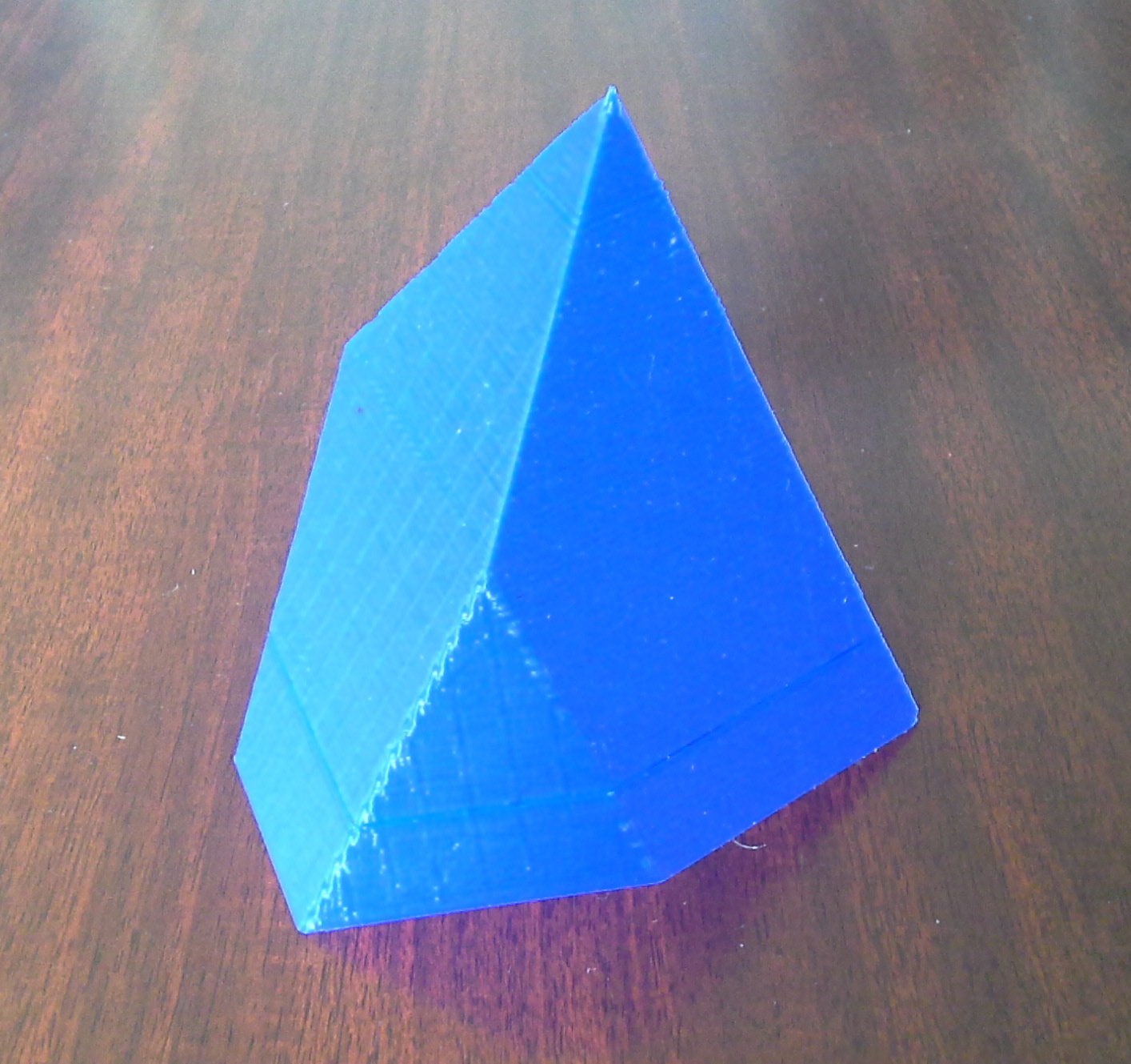
A colleague of mine in the mechanical engineering department, Professor Ron Adrezin, has been getting very active with 3D printers. Along with his colleagues, he has outfitted their labs with numerous 3D printers for use by students and faculty. He was written up last fall in the local newspaper for his work with a 3D printer onboard a Coast Guard Arctic Icebreaker. So when I saw Ron at an in-service day before this semester began, I asked him if he could print a polytope and offered to send him more specifics on the shape I was talking about. I referred him to my greenOR blog post from 2014 “Visualizing LPs in Mathematica“. This email conversation followed:
Ron: Can you save it as an stl file?
Me: never heard of that, but Mathematica can – https://reference.wolfram.com/language/ref/format/STL.html … i exported the polytope as an .stl file – please see attached … thanks!
Ron: Thanks, I will take a look.
A couple of days later Ron let me know his colleague Tom printed it! They used a Makerbot 5th generation 3D printer and the Makerbot software.
Here are a couple of 2D photos of this 3D polytope:

Here is the source in Mathematica:

feasible region in Mathematica
It was a pleasant surprise to learn that the file type the Makerbot software took as input, the .stl file, was something Mathematica could export. See the link above for how to do it.
It’s been fun showing it off to colleagues and using it as a visual aid in Linear Optimization class that students can hold. We’re planning to give students in the class the chance to have theirs printed.
Some google searching digs up a lot of activity on 3D printing mathematical objects. Here are a few I found interesting:
http://www.georgehart.com/rp/rp.html
https://plus.maths.org/content/3d-printing
https://www.simonsfoundation.org/multimedia/3-d-printing-of-mathematical-models/# At 3:37 of video, he shows Mathematica with something that looks like it could be used for an IP feasible region with objective. There’s also mention of the program “stella” which is useful for polyhedra.
3D printers are fairly common at MakerSpaces. Our city of New London has a few at its brand new “Spark” MakerSpace. I am looking forward to more 3D printing to come…
The Capstone is the culminating course in our Operations Research and Computer Analysis (ORCA) undergraduate major. Students work in small teams on applied O.R./Analytics problems. (See this page for links to ones we have done pertaining to sustainability.) Some of the outcomes we have for students through this course are:
- define, formulate and solve an O.R./analytics problem
- use technology and software to aid in problem solving
- read/understand mathematical texts/papers
- write sound technical passages
- prepare and deliver an oral presentation
- work as an effective member of a team
The idea is that these outcomes and others are progressively targeted over the prior 3 1/2 years across the courses leading up to the Capstone. In this way, the students are ready to achieve this final set of culminating outcomes in the Capstone course. And in reality, we do target many goals in earlier courses that support this development. For example, modeling is emphasized in courses such linear optimization, network & nonlinear optimization, decision models, probability models, linear regression, and more. Technical writing and oral presentation projects pop up in various courses along the way. In a program review effort a few years ago, we documented the overall departmental outcomes and the extent to which each was addressed in each course. In an even earlier review in 2000, a matrix of outcomes was created giving a quick visual picture of where the outcomes are addressed over time and how they build. We are due for a review and more refined look at this outcome development.
At Wooster College, seniors undertake an “Independent Study” (IS) in which they come up with a project and are mentored on it by faculty. The whole four-year academic experience at Wooster is geared towards the IS. According to a description in the book Colleges That Change Lives:
Professors infuse every course with a set of skills students must master to be successful researchers: They learn to frame questions, identify reliable sources, analyze primary documents, practice methodologies and write cogently – precisely the skills that are invaluable in the workplace and graduate school. In essence, the curriculum is built backward, starting with a clear vision of what students need to complete IS successfully. That vision guides how professors teach even introductory courses.
The concept of building the curriculum backwards makes a lot of sense to me and we have started having conversations about doing this in our department. In some cases, some of us have noted shortcomings in our students at the Capstone level and tried to address these earlier on in the curriculum in more of an ad hoc fashion. For example, taking a situation that could possibly be modeled a certain way, but that is not presented neatly in textbook form, and bringing it to a formulated model has sometimes been a trouble spot for some students. We have started to incorporate assignments in earlier courses to help address this. The scaffolded project-based learning scheme I spoke about in this webinar (using sustainability as the subject matter) has been a useful paradigm for this effort. We can provide the methodology to be used to the students (e.g., linear programming) but have them supply problem situation complete with parameters, objective, and constraints. On the other hand, late in the curriculum, we can provide a problem with any necessary data, but rely on them to look through their toolboxes for the appropriate methodology. I believe these efforts are beneficial but that they could be even more beneficial if undertaken in a systematic way so as to develop the desired Capstone competencies incrementally throughout the curriculum.
— — — — —
In the book The Mind at Work by Mike Rose, there is a neat passage about a high school woodshop class having students ranging from freshman through seniors that ran like a kind of guild. The teacher was the master craftsman while the seniors had developed an impressive set of skills and experience and could build and/or supervise fairly extensive projects. The freshman were learning the basics, getting hands-on training, absorbing information and concepts from the upper class. Between was a continuum of learning with younger learning from older. I think this would be an effective way to run an O.R. Capstone as well. As they do now, the projects would start with a situation. The students of all the levels wrestle with the intangibles trying to refine it to a problem statement. The upper class familiar with methodology begin to cast the problem in those terms. Mid-level students can do the formulating and start the solving, analysis, coding, etc. under the supervision of the seniors, with the lowest level students pitching in on some of the lower level mechanics involved in these processes. Then all the students work on solution interpretation and an iterative process ensues in which students are involved to varying degrees depending on what their level of training is, but also based on what other things they bring to the table – creativity, hard work, grit, gumption, etc. This could probably be applied in other areas besides the Capstone such as across the core math courses (a differential equations project is going to require skills from pre-calc, calc I, and calc II – so put students from those four courses together on a team), and across the STEAM disciplines, if not beyond. And/or maybe the faculty serve as team members doing work on the project, not just advising. I did a quick google search for this type of situation and came upon “vertically integrated projects”. Georgia Tech has such a program that is multidisciplinary, vertically-integrated (sophomores through PhD students), and long-term. The long-term aspect is another potential bonus in that students can continue work on a large project from year to year but at a deeper level each year. I plan to look more into this notion of vertically-integrated projects and hope to help implement something like it at some point.
Here in Connecticut, the first statewide Campus Sustainability Week is going on this week (October 5th – 9th). It is filled with great events at colleges and universities throughout the state (see the calendar here) such as:
- screening of the documentary Reuse on Thursday at Eastern CT State U. (see below)
- garden cleanup at the Univ. of Hartford on Tuesday
- vegan potluck and movie at Eastern on Wednesday
- Yale farm work day on Friday
and much more…
Here’s the trailer for Reuse:
I put together a poster about the carbon emissions game I’ve mentioned on this blog before to be shown at MathFest. Thanks to Ben Galluzzo from Shippensburg University for arranging for the poster to be shown without me being able to be there. Ben and Corrine Taylor of Wellesley College are co-chairs of “USE Math”, short for Undergraduate Sustainability Experiences in Mathematics. Their mission has a lot in common with what I’ve written about on this blog from the OR/MS perspective:
The carbon game poster is part of USE Math’s poster session “Classroom Activities and Projects within the Context of Environmental Sustainability” to be held Thursday, August 6, 3:30 PM – 5:00 PM. See this page (scroll down) for more information. The full list of poster abstracts is available here (pdf).
If you won’t be at MathFest you can have a look at the poster below. (Click on the image for a larger version.) My game co-developer Bob Day and I have a paper in progress about the game. We also may be taking the game on the road in the future, running it at other schools, conferences, etc. Stay tuned.

Carbon Emissions Game Poster
With all of the energy- and environment-related data now available through sensors, machines, and other equipment there are great possibilities for green O.R. and analytics surrounding the “Internet of Things”. A recent blurb in Harvard Magazine by Stephanie Garlock discusses work of HBS professors Marco Iansiti and Karim R. Lakhani who found many business have undergone serious transformations by actively utilizing data from this new realm. The example of G.E. is mentioned in article:
The “industrial internet” is the term GE executives have coined to refer to these digital integration efforts. The corporation’s new approach to selling wind turbines exemplifies the opportunities and challenges that this connected future presents. Before the world went digital, the easiest way for GE to add value to a customer’s wind farm was to sell it more turbines. Now sensors wirelessly transmit data on performance and maintenance back to GE, which can replace worn-out parts before they break and adjust controls for torque, pitch, and speed in real time. By keeping the turbines running more efficiently, GE has created worth without selling more products—and a new price model allows the company to capture part of this value. Rather than charging for the turbine alone, the sales force can quantify the wind farm’s data-driven savings and charge a fee based on the value of that optimization. These new ways of creating and capturing value have gone hand in hand with fundamental changes in GE’s operations. The company has invested billions in GE Software, and retrained its sales force to focus on long-term contracts and pay-for-performance.

Gene Woolsey (src: http://inside.mines.edu/fs_home/rwoolsey/)
I was saddened to learn in the June issue of ORMS today that Gene Woolsey passed away. There is a poignant “In Memoriam” article about him in that issue with remembrances from former students and colleagues. Gysbert Wessels, a former student of Woolsey’s describes the “OR/MS Guild” in place under Woolsey at the Colorado School of Mines:
Gene’s approach to teaching O.R. was unique. All students sat with him, an open plan without any partitions. As the number of students increased, he had a classroom converted into his office. He taught us not only in classes and by sharing real-life incidents, but just sitting in his office with him exposed us to us dealing with clients, university politics, editing journals, TIMS and ORSA politics, etc.
Wessels closes the article with this statement:
Gene was a teacher and mentor. He thought for himself and taught his students to think. This meant questioning, consulting the original sources, considering the facts and drawing your own conclusions. He made a huge contribution to operations research and management science. He will be missed by his family, friends and students.
Although I never had the good fortune to meet Gene Woolsey, I was influenced by his writings. In 2008, I stumbled upon a copy of the book The Woolsey Papers in our Coast Guard Academy Library.  The lessons in it, particularly the emphasis on practicality, resonated with me. I learned a lot from it that I have tried to apply since then in teaching undergrad O.R. courses, advising capstone projects, and in consulting. See the greenOR posts:
- The Woolsey Papers, Part I
- The Woolsey Papers, Part 2: an application of some of the ideas
- The Woolsey Papers, Part 3: postscripts
Perhaps my favorite quote, which gets at Gene Woolsey’s dedication to service is this one:
In short, I worked for free, so I could work for money, with some hope of gain, so I could afford to choose which pro bono project would be the most fun to do next… This is the tip of the iceberg of what we have done for ourselves and for our state and community. What are you doing for yours?
Here are a few interesting bits and pieces I have come across recently:
 Check out the “Gestión de Operaciones” website. It is a blog on operations management and operations research in Spanish, written by Francisco Yuraszeck, professor in Operational Research at the Universidad Santa Maria in Viña del Mar, Chile. The purpose of the site is to expose students from Spanish speaking countries to the basics and most important topics in these fields.
- A while back I posted a bit about “The Toaster Project” in which Thomas Thwaites attempted to build a toaster from scratch … literally. He went around England’s abandoned mines to extract the metal ore, and so on. The project is now completed and Thwaites has a book about it. See the website. He was on the Colbert Report to talk about it. Thwaites explains how a conventional toaster consists of “400 bits”. The exchange with Colbert was very funny. Colbert: “He even hunted his own bread.” and “Two questions: Why? … and … Why?”
- On this blog I have often harped about the importance of repair of products in sustainability. I have been doing a lot more repair myself recently and have found the resources on the web are very helpful. YouTube has a huge set of videos on repairing all kinds of items. And there is the ifixit site, a big proponent of repair. Their “Repair Jobs Revolution” page is right on the mark: “It’s Time for a Repair Jobs Revolution: Fostering repair will give people access to affordable products, make a huge dent in the e-waste problem, and create jobs.” The .com side of ifixit has repair guides, especially for computers, phones and tablets, and parts and tools for sale.
- The journal OMEGA has a Special Issue on “New Research Frontiers in Sustainability”. The dealine for submission is December 30, 2014. Omega has come up a lot on this blog before. Here is an excerpt from the call for papers:
The aim of this special issue is to publish state-of-the-art research papers which address sustainability problems and challenges on the interface between the three TBL dimensions (profit, people, and planet). Analytical models, empirical studies, and case-based studies are all welcomed as long as an article provides new insights and implications to the practice of management science concerning sustainability.

